Comparing observations to emissions

In this tutorial, we will see how to combine observation data and acillary data into a ModelScenario, which can compute modelled outputs based on ancillary data, and compare these modelled outputs to observed measurements.

This tutorial builds on the tutorials Adding observation data and Adding ancillary spatial data.

Note

Plots created within this tutorial may not show up on the online documentation version of this notebook.

Using the tutorial object store

As in the previous tutorials, we will use the tutorial object store to avoid cluttering your personal object store.

from openghg.tutorial import use_tutorial_store

use_tutorial_store()

Omit this step if you want to analyse data in your local object store. (This data needs to be added following the instructions in the previous tutorials.)

1. Loading data sources into the object store

We begin by adding observation, footprint, flux, and (optionally) boundary conditions data to the object store. See Adding ancillary spatial data for more details on these inputs. This data relates to Tacolneston (TAC) site within the DECC network and the area around Europe (EUROPE domain).

We’ll use some helper functions from the openghg.tutorial submodule to retrieve raw data in the expected format:

from openghg.tutorial import populate_surface_data, populate_footprint_inert, populate_flux_ch4, populate_bc_ch4

populate_surface_data()

populate_footprint_inert()

populate_flux_ch4()

populate_bc_ch4()

2. Creating a model scenario

With this ancillary data, we can start to make comparisons between model data, such as bottom-up inventories, and our observations. This analysis is based around a ModelScenario object which can be created to link together observation, footprint, flux / emissions data and boundary conditions data.

Above we loaded observation data from the Tacolneston site into the object store. We also added both an associated footprint (sensitivity map) and an anthropogenic emissions map for a domain defined over Europe.

To access and link this data we can set up our ModelScenario instance using a similar set of keywords. In this case we have also limited ourselves to a date range:

from openghg.analyse import ModelScenario

species="ch4"
site="tac"
domain="EUROPE"
height="100m"
source_waste = "waste"
start_date = "2016-07-01"
end_date = "2016-08-01"

scenario = ModelScenario(site=site,
                         inlet=height,
                         domain=domain,
                         species=species,
                         source=source_waste,
                         start_date=start_date,
                         end_date=end_date)

                    INFO     INFO:openghg.analyse:Adding obs_surface to model scenario             _scenario.py:335

                    INFO     INFO:openghg.analyse:Updating any inputs based on observation data    _scenario.py:240

                    INFO     INFO:openghg.analyse:site: tac, species: ch4, inlet: 100m             _scenario.py:241

                    INFO     INFO:openghg.analyse:Using height_name option(s) for footprint inlet: _scenario.py:477
                             100magl.                                                                              
                             Inferred from site=tac, network=decc, inlet=100m                                      

                    INFO     INFO:openghg.analyse:Adding footprint to model scenario               _scenario.py:335

                    INFO     INFO:openghg.analyse:Adding flux to model scenario                    _scenario.py:335

                    INFO     INFO:openghg.analyse:Adding boundary_conditions to model scenario     _scenario.py:335

Using these keywords, this will search the object store and attempt to collect and attach observation, footprint, flux and boundary conditions data. This collected data will be attached to your created ModelScenario. For the observations this will be stored as the ModelScenario.obs attribute. This will be an ObsData object which contains metadata and data for your observations:

scenario.obs

ObsData(metadata={'site': 'tac', 'instrument': 'picarro', 'sampling_period': '3600.0', 'inlet': '100m', ...}, uuid=c3db13a3-74ce-4944-9ac1-90ab563b9a23)

To access the undelying xarray Dataset containing the observation data use ModelScenario.obs.data:

scenario.obs.data

<xarray.Dataset> Size: 19kB
Dimensions:                    (time: 608)
Coordinates:
  * time                       (time) datetime64[ns] 5kB 2016-07-01T00:18:58 ...
Data variables:
    mf                         (time) float64 5kB dask.array<chunksize=(608,), meta=np.ndarray>
    mf_number_of_observations  (time) int64 5kB dask.array<chunksize=(608,), meta=np.ndarray>
    mf_variability             (time) float64 5kB dask.array<chunksize=(608,), meta=np.ndarray>
Attributes: (12/27)
    Conventions:           CF-1.8
    comment:               Cavity ring-down measurements. Output from GCWerks
    conditions_of_use:     Ensure that you contact the data owner at the outs...
    data_owner:            Simon O'Doherty
    data_owner_email:      s.odoherty@bristol.ac.uk
    data_source:           internal
    ...                    ...
    station_height_masl:   64
    station_latitude:      52.51882
    station_long_name:     Tacolneston Tower, UK
    station_longitude:     1.1387
    type:                  air
    scale:                 WMO-X2004A

xarray.Dataset

• Dimensions:
  • time: 608
• Coordinates: (1)
  • time
    (time)
    datetime64[ns]
    2016-07-01T00:18:58 ... 2016-07-...

    comment :

    Time stamp corresponds to beginning of sampling period. Time since midnight UTC of reference date. Note that sampling periods are approximate.

    label :

    left

    sampling_period_seconds :

    3600.0

    standard_name :

    time

    array(['2016-07-01T00:18:58.000000000', '2016-07-01T01:38:58.000000000',
           '2016-07-01T02:39:02.000000000', ..., '2016-07-28T18:37:06.000000000',
           '2016-07-28T19:37:09.000000000', '2016-07-28T20:37:08.000000000'],
          shape=(608,), dtype='datetime64[ns]')

• Data variables: (3)
  • mf
    (time)
    float64
    dask.array<chunksize=(608,), meta=np.ndarray>

    long_name :

    mole_fraction_of_methane_in_air

    units :

    1e-9

    Array Chunk Bytes 4.75 kiB 4.75 kiB Shape (608,) (608,) Dask graph 1 chunks in 5 graph layers Data type float64 numpy.ndarray

  • mf_number_of_observations
    (time)
    int64
    dask.array<chunksize=(608,), meta=np.ndarray>

    long_name :

    mole_fraction_of_methane_in_air_number_of_observations

    Array Chunk Bytes 4.75 kiB 4.75 kiB Shape (608,) (608,) Dask graph 1 chunks in 5 graph layers Data type int64 numpy.ndarray

  • mf_variability
    (time)
    float64
    dask.array<chunksize=(608,), meta=np.ndarray>

    long_name :

    mole_fraction_of_methane_in_air_variability

    units :

    1e-9

    Array Chunk Bytes 4.75 kiB 4.75 kiB Shape (608,) (608,) Dask graph 1 chunks in 5 graph layers Data type float64 numpy.ndarray

• Attributes: (27)

  Conventions :

  CF-1.8

  comment :

  Cavity ring-down measurements. Output from GCWerks

  conditions_of_use :

  Ensure that you contact the data owner at the outset of your project.

  data_owner :

  Simon O'Doherty

  data_owner_email :

  s.odoherty@bristol.ac.uk

  data_source :

  internal

  data_type :

  surface

  file_created :

  2025-11-15 21:14:34.263739+00:00

  inlet :

  100m

  inlet_height_magl :

  100

  instrument :

  picarro

  long_name :

  tacolneston

  network :

  decc

  port :

  9

  processed_by :

  OpenGHG_Cloud

  sampling_period :

  3600.0

  sampling_period_unit :

  s

  site :

  tac

  source :

  In situ measurements of air

  source_format :

  CRDS

  species :

  ch4

  station_height_masl :

  64

  station_latitude :

  52.51882

  station_long_name :

  Tacolneston Tower, UK

  station_longitude :

  1.1387

  type :

  air

  scale :

  WMO-X2004A

The ModelScenario.footprint attribute contains the linked FootprintData (again, use .data to extract xarray Dataset):

scenario.footprint

FootprintData(metadata={'site': 'tac', 'domain': 'europe', 'model': 'name', 'inlet': '100m', ...}, uuid=5e44feea-933e-46b3-b96b-43875eca0bbe)

And the ModelScenario.fluxes attribute can be used to access the FluxData. Note that for ModelScenario.fluxes this can contain multiple flux sources and so this is stored as a dictionary linked to the source name:

scenario.fluxes

{'waste': FluxData(metadata={'raw file used': '/home/cv18710/work_shared/gridded_fluxes/ch4/ukghg/uk_flux_waste_ch4_lonlat_0.01km_2016.nc', 'species': 'ch4', 'domain': 'europe', 'source': 'waste', ...}, uuid=d85145a0-4a6d-40c3-b6a8-87ddd1a8bb11)}

Finally, this will also search and attempt to add boundary conditions. The ModelScenario.bc attribute can be used to access the BoundaryConditionsData if present.

scenario.bc

BoundaryConditionsData(metadata={'date_created': '2018-11-13 09:25:29.112138', 'species': 'ch4', 'domain': 'europe', 'bc_input': 'cams', ...}, uuid=505eade0-5621-411c-a1ff-523194be4455)

scenario.bc.data.attrs

{'author': 'OpenGHG Cloud',
 'bc_input': 'cams',
 'date_created': '2018-11-13 09:25:29.112138',
 'domain': 'europe',
 'end_date': '2016-07-31 23:59:59+00:00',
 'max_height': 19500.0,
 'max_latitude': 79.057,
 'max_longitude': 39.38,
 'min_height': 500.0,
 'min_latitude': 10.729,
 'min_longitude': -97.9,
 'processed': '2025-11-15 21:14:54.094062+00:00',
 'species': 'ch4',
 'start_date': '2016-07-01 00:00:00+00:00',
 'time_period': '1 month',
 'title': 'ECMWF CAMS ch4 volume mixing ratios at domain edges'}

An interactive plot for the linked observation data can be plotted using the ModelScenario.plot_timeseries() method:

scenario.plot_timeseries()

You can also set up your own searches and add this data directly. One benefit of this interface is to reduce searching the database if the same data needs to be used for multiple different scenarios.

from openghg.retrieve import get_obs_surface, get_footprint, get_flux, get_bc

# Extract obs results from object store
obs_results = get_obs_surface(site=site,
                              species=species,
                              inlet=height,
                              start_date="2016-07-01",
                              end_date="2016-08-01")

# Extract footprint results from object store
footprint_results = get_footprint(site=site,
                                  domain=domain,
                                  height=height,
                                  start_date="2016-07-01",
                                  end_date="2016-08-01")

# Extract flux results from object store
flux_results = get_flux(species=species,
                        domain=domain,
                        source=source_waste,
                        start_date="2016-01-01",
                        end_date="2016-12-31")

# Extract specific boundary conditions from the object store
bc_results = get_bc(species=species,
                    domain=domain,
                    bc_input="CAMS",
                    start_date="2016-07-01",
                    end_date="2016-08-01")

scenario_direct = ModelScenario(obs=obs_results, footprint=footprint_results, flux=flux_results, bc=bc_results)

2025-11-15T21:14:56 INFO     INFO:openghg.analyse:Updating any inputs based on observation data    _scenario.py:240

                    INFO     INFO:openghg.analyse:site: tac, species: ch4, inlet: 100m             _scenario.py:241

Note

You can create your own input objects directly and add these in the same way. This allows you to bypass the object store for experimental examples. At the moment these inputs need to be ObsData, FootprintData, FluxData or BoundaryConditionsData objects, which can be created using classes from openghg.dataobjects. Simpler inputs will be made available.

3. Comparing data sources

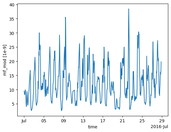
Once your ModelScenario has been created you can then start to use the linked data to compare outputs. For example we may want to calculate modelled observations at our site based on our linked footprint and emissions data:

modelled_observations = scenario.calc_modelled_obs()

                    INFO     INFO:openghg.analyse:Platform of 'None' for site 'tac' extracted from _scenario.py:771
                             site_info.json                                                                        

2025-11-15T21:14:57 INFO     INFO:openghg.analyse:Caching calculated data                         _scenario.py:1159

This could then be plotted directly using the xarray plotting methods:

modelled_observations.mf_mod.plot()  # Can plot using xarray plotting methods

[<matplotlib.lines.Line2D at 0x7f6bb6728950>]

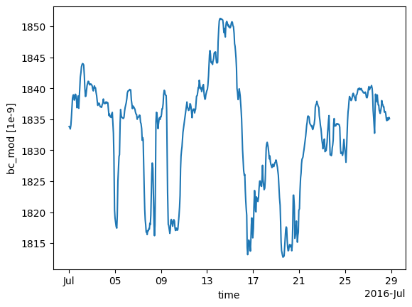
The modelled baseline, based on the linked boundary conditions, can also be calculated in a similar way:

modelled_baseline = scenario.calc_modelled_baseline()
modelled_baseline.bc_mod.plot()  # Can plot using xarray plotting methods

2025-11-15T21:14:59 INFO     INFO:openghg.analyse:Caching calculated data                         _scenario.py:1358

[<matplotlib.lines.Line2D at 0x7f6ba6331a60>]

To compare these modelled observations to the observations themselves, the ModelScenario.plot_comparison() method can be used. This will stack the modelled observations and the modelled baseline by default to allow comparison:

scenario.plot_comparison()

2025-11-15T21:15:04 INFO     INFO:openghg.analyse:Caching calculated data                         _scenario.py:1358

The ModelScenario.footprints_data_merge() method can also be used to created a combined output, with all aligned data stored directly within an xarray.Dataset:

combined_dataset = scenario.footprints_data_merge()
combined_dataset

2025-11-15T21:15:14 INFO     INFO:openghg.analyse:Caching calculated data                         _scenario.py:1358

<xarray.Dataset> Size: 412MB
Dimensions:                              (time: 608, lat: 293, lon: 391,
                                          height: 20)
Coordinates:
  * time                                 (time) datetime64[ns] 5kB 2016-07-01...
  * height                               (height) float32 80B 500.0 ... 1.95e+04
  * lat                                  (lat) float64 2kB 10.73 10.96 ... 79.06
  * lon                                  (lon) float64 3kB -97.9 ... 39.38
Data variables: (12/22)
    mf                                   (time) float64 5kB dask.array<chunksize=(608,), meta=np.ndarray>
    mf_number_of_observations            (time) float64 5kB dask.array<chunksize=(608,), meta=np.ndarray>
    mf_variability                       (time) float64 5kB dask.array<chunksize=(608,), meta=np.ndarray>
    air_pressure                         (time) float32 2kB dask.array<chunksize=(335,), meta=np.ndarray>
    air_temperature                      (time) float32 2kB dask.array<chunksize=(335,), meta=np.ndarray>
    atmosphere_boundary_layer_thickness  (time) float32 2kB dask.array<chunksize=(335,), meta=np.ndarray>
    ...                                   ...
    release_lat                          (time) float32 2kB dask.array<chunksize=(335,), meta=np.ndarray>
    release_lon                          (time) float32 2kB dask.array<chunksize=(335,), meta=np.ndarray>
    wind_from_direction                  (time) float32 2kB dask.array<chunksize=(335,), meta=np.ndarray>
    wind_speed                           (time) float32 2kB dask.array<chunksize=(335,), meta=np.ndarray>
    mf_mod                               (time) float32 2kB dask.array<chunksize=(335,), meta=np.ndarray>
    bc_mod                               (time) float32 2kB dask.array<chunksize=(1,), meta=np.ndarray>
Attributes: (12/45)
    Conventions:              CF-1.8
    comment:                  Cavity ring-down measurements. Output from GCWerks
    conditions_of_use:        Ensure that you contact the data owner at the o...
    data_owner:               Simon O'Doherty
    data_owner_email:         s.odoherty@bristol.ac.uk
    data_source:              internal
    ...                       ...
    short_lifetime:           False
    start_date:               2016-07-01 00:00:00+00:00
    time_period:              1 hour
    time_resolved:            False
    variables:                ['fp', 'air_temperature', 'air_pressure', 'wind...
    resample_to:              coarsest

xarray.Dataset

• Dimensions:
  • time: 608
  • lat: 293
  • lon: 391
  • height: 20
• Coordinates: (4)
  • time
    (time)
    datetime64[ns]
    2016-07-01T00:18:58 ... 2016-07-...

    comment :

    Time stamp corresponds to beginning of sampling period. Time since midnight UTC of reference date. Note that sampling periods are approximate.

    label :

    left

    sampling_period_seconds :

    3600.0

    standard_name :

    time

    array(['2016-07-01T00:18:58.000000000', '2016-07-01T01:38:58.000000000',
           '2016-07-01T02:39:02.000000000', ..., '2016-07-28T18:37:06.000000000',
           '2016-07-28T19:37:09.000000000', '2016-07-28T20:37:08.000000000'],
          shape=(608,), dtype='datetime64[ns]')

  • height
    (height)
    float32
    500.0 1.5e+03 ... 1.85e+04 1.95e+04

    least_significant_digit :

    4

    array([  500.,  1500.,  2500.,  3500.,  4500.,  5500.,  6500.,  7500.,  8500.,
            9500., 10500., 11500., 12500., 13500., 14500., 15500., 16500., 17500.,
           18500., 19500.], dtype=float32)

  • lat
    (lat)
    float64
    10.73 10.96 11.2 ... 78.82 79.06

    units :

    degrees_north

    array([10.729   , 10.963   , 11.197   , ..., 78.588997, 78.822998, 79.056999],
          shape=(293,))

  • lon
    (lon)
    float64
    -97.9 -97.55 -97.2 ... 39.03 39.38

    units :

    degrees_east

    array([-97.900002, -97.547997, -97.195999, ...,  38.675999,  39.028   ,
            39.380001], shape=(391,))

• Data variables: (22)
  • mf
    (time)
    float64
    dask.array<chunksize=(608,), meta=np.ndarray>

    long_name :

    mole_fraction_of_methane_in_air

    units :

    1e-9

    Array Chunk Bytes 4.75 kiB 4.75 kiB Shape (608,) (608,) Dask graph 1 chunks in 8 graph layers Data type float64 numpy.ndarray

  • mf_number_of_observations
    (time)
    float64
    dask.array<chunksize=(608,), meta=np.ndarray>

    long_name :

    mole_fraction_of_methane_in_air_number_of_observations

    Array Chunk Bytes 4.75 kiB 4.75 kiB Shape (608,) (608,) Dask graph 1 chunks in 9 graph layers Data type float64 numpy.ndarray

  • mf_variability
    (time)
    float64
    dask.array<chunksize=(608,), meta=np.ndarray>

    long_name :

    mole_fraction_of_methane_in_air_variability

    units :

    1e-9

    Array Chunk Bytes 4.75 kiB 4.75 kiB Shape (608,) (608,) Dask graph 1 chunks in 8 graph layers Data type float64 numpy.ndarray

  • air_pressure
    (time)
    float32
    dask.array<chunksize=(335,), meta=np.ndarray>

    least_significant_digit :

    4

    long_name :

    air pressure at release

    units :

    hectopascal

    Array Chunk Bytes 2.38 kiB 1.31 kiB Shape (608,) (335,) Dask graph 2 chunks in 10 graph layers Data type float32 numpy.ndarray

  • air_temperature
    (time)
    float32
    dask.array<chunksize=(335,), meta=np.ndarray>

    least_significant_digit :

    4

    long_name :

    air temperature at release

    units :

    °C

    Array Chunk Bytes 2.38 kiB 1.31 kiB Shape (608,) (335,) Dask graph 2 chunks in 10 graph layers Data type float32 numpy.ndarray

  • atmosphere_boundary_layer_thickness
    (time)
    float32
    dask.array<chunksize=(335,), meta=np.ndarray>

    least_significant_digit :

    4

    long_name :

    atmospheric boundary layer thickness at release

    units :

    m

    Array Chunk Bytes 2.38 kiB 1.31 kiB Shape (608,) (335,) Dask graph 2 chunks in 10 graph layers Data type float32 numpy.ndarray

  • fp
    (lat, lon, time)
    float32
    dask.array<chunksize=(293, 391, 335), meta=np.ndarray>

    least_significant_digit :

    5

    long_name :

    source_receptor_relationship

    loss_lifetime_hrs :

    No loss applied

    units :

    m2 s mol-1

    Array Chunk Bytes 265.71 MiB 146.40 MiB Shape (293, 391, 608) (293, 391, 335) Dask graph 2 chunks in 11 graph layers Data type float32 numpy.ndarray

  • mean_age_particles_e
    (height, lat, time)
    float32
    dask.array<chunksize=(20, 293, 335), meta=np.ndarray>

    least_significant_digit :

    7

    long_name :

    Mean age of particles leaving domain (E side)

    units :

    h

    Array Chunk Bytes 13.59 MiB 7.49 MiB Shape (20, 293, 608) (20, 293, 335) Dask graph 2 chunks in 11 graph layers Data type float32 numpy.ndarray

  • mean_age_particles_n
    (height, lon, time)
    float32
    dask.array<chunksize=(20, 391, 335), meta=np.ndarray>

    least_significant_digit :

    7

    long_name :

    Mean age of particles leaving domain (N side)

    units :

    h

    Array Chunk Bytes 18.14 MiB 9.99 MiB Shape (20, 391, 608) (20, 391, 335) Dask graph 2 chunks in 11 graph layers Data type float32 numpy.ndarray

  • mean_age_particles_s
    (height, lon, time)
    float32
    dask.array<chunksize=(20, 391, 335), meta=np.ndarray>

    least_significant_digit :

    7

    long_name :

    Mean age of particles leaving domain (S side)

    units :

    h

    Array Chunk Bytes 18.14 MiB 9.99 MiB Shape (20, 391, 608) (20, 391, 335) Dask graph 2 chunks in 11 graph layers Data type float32 numpy.ndarray

  • mean_age_particles_w
    (height, lat, time)
    float32
    dask.array<chunksize=(20, 293, 335), meta=np.ndarray>

    least_significant_digit :

    7

    long_name :

    Mean age of particles leaving domain (W side)

    units :

    h

    Array Chunk Bytes 13.59 MiB 7.49 MiB Shape (20, 293, 608) (20, 293, 335) Dask graph 2 chunks in 11 graph layers Data type float32 numpy.ndarray

  • particle_locations_e
    (height, lat, time)
    float32
    dask.array<chunksize=(20, 293, 335), meta=np.ndarray>

    least_significant_digit :

    7

    long_name :

    Fraction of total particles leaving domain (E side)

    units :

    1

    Array Chunk Bytes 13.59 MiB 7.49 MiB Shape (20, 293, 608) (20, 293, 335) Dask graph 2 chunks in 11 graph layers Data type float32 numpy.ndarray

  • particle_locations_n
    (height, lon, time)
    float32
    dask.array<chunksize=(20, 391, 335), meta=np.ndarray>

    least_significant_digit :

    7

    long_name :

    Fraction of total particles leaving domain (N side)

    units :

    1

    Array Chunk Bytes 18.14 MiB 9.99 MiB Shape (20, 391, 608) (20, 391, 335) Dask graph 2 chunks in 11 graph layers Data type float32 numpy.ndarray

  • particle_locations_s
    (height, lon, time)
    float32
    dask.array<chunksize=(20, 391, 335), meta=np.ndarray>

    least_significant_digit :

    7

    long_name :

    Fraction of total particles leaving domain (S side)

    units :

    1

    Array Chunk Bytes 18.14 MiB 9.99 MiB Shape (20, 391, 608) (20, 391, 335) Dask graph 2 chunks in 11 graph layers Data type float32 numpy.ndarray

  • particle_locations_w
    (height, lat, time)
    float32
    dask.array<chunksize=(20, 293, 335), meta=np.ndarray>

    least_significant_digit :

    7

    long_name :

    Fraction of total particles leaving domain (W side)

    units :

    1

    Array Chunk Bytes 13.59 MiB 7.49 MiB Shape (20, 293, 608) (20, 293, 335) Dask graph 2 chunks in 11 graph layers Data type float32 numpy.ndarray

  • release_height
    (time)
    float64
    dask.array<chunksize=(335,), meta=np.ndarray>

    long_name :

    Release height above model ground

    units :

    m

    Array Chunk Bytes 4.75 kiB 2.62 kiB Shape (608,) (335,) Dask graph 2 chunks in 11 graph layers Data type float64 numpy.ndarray

  • release_lat
    (time)
    float32
    dask.array<chunksize=(335,), meta=np.ndarray>

    least_significant_digit :

    4

    long_name :

    Release latitude

    units :

    degrees_north

    Array Chunk Bytes 2.38 kiB 1.31 kiB Shape (608,) (335,) Dask graph 2 chunks in 10 graph layers Data type float32 numpy.ndarray

  • release_lon
    (time)
    float32
    dask.array<chunksize=(335,), meta=np.ndarray>

    least_significant_digit :

    4

    long_name :

    Release longitude

    units :

    degrees_east

    Array Chunk Bytes 2.38 kiB 1.31 kiB Shape (608,) (335,) Dask graph 2 chunks in 10 graph layers Data type float32 numpy.ndarray

  • wind_from_direction
    (time)
    float32
    dask.array<chunksize=(335,), meta=np.ndarray>

    least_significant_digit :

    4

    long_name :

    wind direction at release

    units :

    deg

    Array Chunk Bytes 2.38 kiB 1.31 kiB Shape (608,) (335,) Dask graph 2 chunks in 10 graph layers Data type float32 numpy.ndarray

  • wind_speed
    (time)
    float32
    dask.array<chunksize=(335,), meta=np.ndarray>

    least_significant_digit :

    4

    long_name :

    wind speed at release

    units :

    m s-1

    Array Chunk Bytes 2.38 kiB 1.31 kiB Shape (608,) (335,) Dask graph 2 chunks in 10 graph layers Data type float32 numpy.ndarray

  • mf_mod
    (time)
    float32
    dask.array<chunksize=(335,), meta=np.ndarray>

    units :

    1e-9

    Array Chunk Bytes 2.38 kiB 1.31 kiB Shape (608,) (335,) Dask graph 2 chunks in 25 graph layers Data type float32 numpy.ndarray

  • bc_mod
    (time)
    float32
    dask.array<chunksize=(1,), meta=np.ndarray>

    resample_to :

    coarsest

    units :

    1e-9

    Array Chunk Bytes 2.38 kiB 4 B Shape (608,) (1,) Dask graph 608 chunks in 99 graph layers Data type float32 numpy.ndarray

• Attributes: (45)

  Conventions :

  CF-1.8

  comment :

  Cavity ring-down measurements. Output from GCWerks

  conditions_of_use :

  Ensure that you contact the data owner at the outset of your project.

  data_owner :

  Simon O'Doherty

  data_owner_email :

  s.odoherty@bristol.ac.uk

  data_source :

  internal

  data_type :

  surface

  file_created :

  2025-11-15 21:14:34.263739+00:00

  inlet :

  100m

  inlet_height_magl :

  100

  instrument :

  picarro

  long_name :

  tacolneston

  network :

  decc

  port :

  9

  processed_by :

  OpenGHG_Cloud

  sampling_period :

  3600.0

  sampling_period_unit :

  s

  site :

  tac

  source :

  In situ measurements of air

  source_format :

  CRDS

  species :

  ch4

  station_height_masl :

  64

  station_latitude :

  52.51882

  station_long_name :

  Tacolneston Tower, UK

  station_longitude :

  1.1387

  type :

  air

  scale :

  WMO-X2004A

  author :

  OpenGHG Cloud

  domain :

  europe

  end_date :

  2016-07-31 23:59:59+00:00

  height :

  100m

  heights :

  [500.0, 1500.0, 2500.0, 3500.0, 4500.0, 5500.0, 6500.0, 7500.0, 8500.0, 9500.0, 10500.0, 11500.0, 12500.0, 13500.0, 14500.0, 15500.0, 16500.0, 17500.0, 18500.0, 19500.0]

  high_spatial_resolution :

  False

  max_latitude :

  79.057

  max_longitude :

  39.38

  min_latitude :

  10.729

  min_longitude :

  -97.9

  model :

  NAME

  processed :

  2025-11-15 21:14:37.548581+00:00

  short_lifetime :

  False

  start_date :

  2016-07-01 00:00:00+00:00

  time_period :

  1 hour

  time_resolved :

  False

  variables :

  ['fp', 'air_temperature', 'air_pressure', 'wind_speed', 'wind_from_direction', 'atmosphere_boundary_layer_thickness', 'release_lon', 'release_lat', 'particle_locations_n', 'particle_locations_e', 'particle_locations_s', 'particle_locations_w', 'mean_age_particles_n', 'mean_age_particles_e', 'mean_age_particles_s', 'mean_age_particles_w', 'release_height']

  resample_to :

  coarsest

When the same calculation is being performed for multiple methods, the last calculation is cached to allow the outputs to be produced more efficiently. This can be disabled for large datasets by using cache=False.

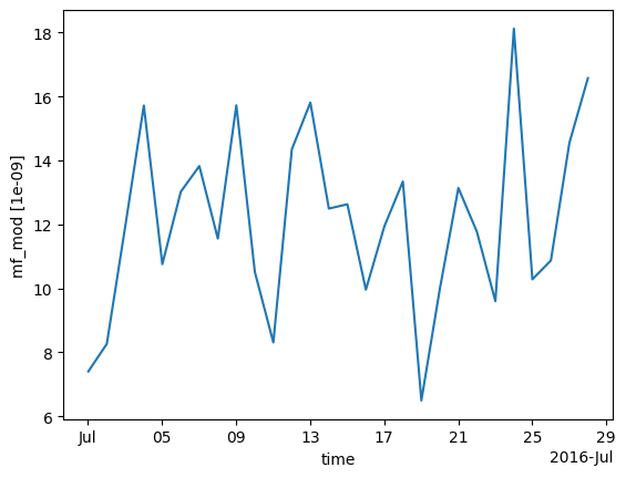
For a ModelScenario object, different analyses can be performed on this linked data. For example if a daily average for the modelled observations was required, we could calculate this by setting our resample_to input to "1D" (matching available pandas time aliases):

modelled_observations_daily = scenario.calc_modelled_obs(resample_to="1D")
modelled_observations_daily.mf_mod.plot()

                    INFO     INFO:openghg.analyse:Platform of 'None' for site 'tac' extracted from _scenario.py:771
                             site_info.json                                                                        

2025-11-15T21:15:15 INFO     INFO:openghg.analyse:Caching calculated data                         _scenario.py:1159

[<matplotlib.lines.Line2D at 0x7f6bb6fe85c0>]

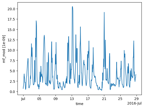
Explicit resampling of the data can be also be skipped by using a resample_to input of None. This will align the footprints to the observations by forward filling the footprint values. Note: using platform="flask" will turn on this option as well.

modelled_observations_align = scenario.calc_modelled_obs(resample_to=None)
modelled_observations_align.mf_mod.plot()

                    INFO     INFO:openghg.analyse:Platform of 'None' for site 'tac' extracted from _scenario.py:771
                             site_info.json                                                                        

2025-11-15T21:15:16 INFO     INFO:openghg.analyse:Caching calculated data                         _scenario.py:1159

[<matplotlib.lines.Line2D at 0x7f6bac3ef0e0>]

To allow comparisons with multiple flux sources, more than one flux source can be linked to your ModelScenario. This can be either be done upon creation or can be added using the add_flux() method. When calculating modelled observations, these flux sources will be aligned in time and stacked to create a total output:

scenario.add_flux(species=species, domain=domain, source="energyprod")

                    INFO     INFO:openghg.analyse:Adding flux to model scenario                    _scenario.py:335

scenario.plot_comparison()

                    INFO     INFO:openghg.analyse:Platform of 'None' for site 'tac' extracted from _scenario.py:771
                             site_info.json                                                                        

2025-11-15T21:15:17 INFO     INFO:openghg.analyse:Caching calculated data                         _scenario.py:1159

                    INFO     INFO:openghg.analyse:Caching calculated data                         _scenario.py:1358

Output for individual sources can also be created by specifying the sources as an input:

# Included recalculate option to ensure this is updated from cached data.
modelled_obs_energyprod = scenario.calc_modelled_obs(sources="energyprod", recalculate=True)
modelled_obs_energyprod.mf_mod.plot()

2025-11-15T21:15:27 INFO     INFO:openghg.analyse:Platform of 'None' for site 'tac' extracted from _scenario.py:771
                             site_info.json                                                                        

2025-11-15T21:15:28 INFO     INFO:openghg.analyse:Caching calculated data                         _scenario.py:1159

[<matplotlib.lines.Line2D at 0x7f6ba691baa0>]

Plotting functions to be added for 2D / 3D data

4. Sensitivity matrices

To perform an inversion for a scenario, we need sensitivity matrices that combine the footprints and flux (or particle locations and boundary conditions). We can get the “footprint x flux” matrix from calc_modelled_obs:

# use the output_fp_x_flux option, which stores the result in the fp_x_flux data variable
# we are recalculating to avoid using cached data
fp_x_flux = scenario.calc_modelled_obs(output_fp_x_flux=True, recalculate=True).fp_x_flux
fp_x_flux

                    INFO     INFO:openghg.analyse:Platform of 'None' for site 'tac' extracted from _scenario.py:771
                             site_info.json                                                                        

2025-11-15T21:15:29 INFO     INFO:openghg.analyse:Caching calculated data                         _scenario.py:1159

<xarray.DataArray 'fp_x_flux' (lat: 293, lon: 391, time: 608)> Size: 279MB
dask.array<mul, shape=(293, 391, 608), dtype=float32, chunksize=(293, 391, 335), chunktype=numpy.ndarray>
Coordinates:
  * time     (time) datetime64[ns] 5kB 2016-07-01T00:18:58 ... 2016-07-28T20:...
  * lat      (lat) float64 2kB 10.73 10.96 11.2 11.43 ... 78.59 78.82 79.06
  * lon      (lon) float64 3kB -97.9 -97.55 -97.2 -96.84 ... 38.68 39.03 39.38
Attributes:
    units:    1e-9

xarray.DataArray

'fp_x_flux'

• lat: 293
• lon: 391
• time: 608

• dask.array<chunksize=(293, 391, 335), meta=np.ndarray>

  Array Chunk Bytes 265.71 MiB 146.40 MiB Shape (293, 391, 608) (293, 391, 335) Dask graph 2 chunks in 27 graph layers Data type float32 numpy.ndarray

• Coordinates: (3)
  • time
    (time)
    datetime64[ns]
    2016-07-01T00:18:58 ... 2016-07-...

    comment :

    Time stamp corresponds to beginning of sampling period. Time since midnight UTC of reference date. Note that sampling periods are approximate.

    label :

    left

    sampling_period_seconds :

    3600.0

    standard_name :

    time

    array(['2016-07-01T00:18:58.000000000', '2016-07-01T01:38:58.000000000',
           '2016-07-01T02:39:02.000000000', ..., '2016-07-28T18:37:06.000000000',
           '2016-07-28T19:37:09.000000000', '2016-07-28T20:37:08.000000000'],
          shape=(608,), dtype='datetime64[ns]')

  • lat
    (lat)
    float64
    10.73 10.96 11.2 ... 78.82 79.06

    units :

    degrees_north

    array([10.729   , 10.963   , 11.197   , ..., 78.588997, 78.822998, 79.056999],
          shape=(293,))

  • lon
    (lon)
    float64
    -97.9 -97.55 -97.2 ... 39.03 39.38

    units :

    degrees_east

    array([-97.900002, -97.547997, -97.195999, ...,  38.675999,  39.028   ,
            39.380001], shape=(391,))

• Attributes: (1)

  units :

  1e-9

To get a matrix suitable for typical inversion frameworks, we can flatten the latitude and longitude coordinates, and use the resulting values.

h = fp_x_flux.stack(latlon=["lat", "lon"]).values

(Normally you would apply basis functions to reduce the size of the matrix.)

The corresponding calculation for baseline sensitivities from boundary conditions is:

from openghg.analyse._modelled_baseline import baseline_sensitivities

bc_sensitivity = scenario.calc_modelled_baseline(output_sensitivity=True)
bc_sensitivity

                    INFO     INFO:openghg.analyse:Caching calculated data                         _scenario.py:1358

<xarray.Dataset> Size: 67MB
Dimensions:  (height: 20, lon: 391, time: 608, lat: 293)
Coordinates:
  * time     (time) datetime64[ns] 5kB 2016-07-01T00:18:58 ... 2016-07-28T20:...
  * height   (height) float32 80B 500.0 1.5e+03 2.5e+03 ... 1.85e+04 1.95e+04
  * lon      (lon) float64 3kB -97.9 -97.55 -97.2 -96.84 ... 38.68 39.03 39.38
  * lat      (lat) float64 2kB 10.73 10.96 11.2 11.43 ... 78.59 78.82 79.06
Data variables:
    bc_n     (height, lon, time) float32 19MB dask.array<chunksize=(20, 391, 1), meta=np.ndarray>
    bc_e     (height, lat, time) float32 14MB dask.array<chunksize=(20, 293, 1), meta=np.ndarray>
    bc_s     (height, lon, time) float32 19MB dask.array<chunksize=(20, 391, 1), meta=np.ndarray>
    bc_w     (height, lat, time) float32 14MB dask.array<chunksize=(20, 293, 1), meta=np.ndarray>
    bc_mod   (time) float32 2kB dask.array<chunksize=(1,), meta=np.ndarray>

xarray.Dataset

• Dimensions:
  • height: 20
  • lon: 391
  • time: 608
  • lat: 293
• Coordinates: (4)
  • time
    (time)
    datetime64[ns]
    2016-07-01T00:18:58 ... 2016-07-...

    comment :

    Time stamp corresponds to beginning of sampling period. Time since midnight UTC of reference date. Note that sampling periods are approximate.

    label :

    left

    sampling_period_seconds :

    3600.0

    standard_name :

    time

    array(['2016-07-01T00:18:58.000000000', '2016-07-01T01:38:58.000000000',
           '2016-07-01T02:39:02.000000000', ..., '2016-07-28T18:37:06.000000000',
           '2016-07-28T19:37:09.000000000', '2016-07-28T20:37:08.000000000'],
          shape=(608,), dtype='datetime64[ns]')

  • height
    (height)
    float32
    500.0 1.5e+03 ... 1.85e+04 1.95e+04

    least_significant_digit :

    4

    array([  500.,  1500.,  2500.,  3500.,  4500.,  5500.,  6500.,  7500.,  8500.,
            9500., 10500., 11500., 12500., 13500., 14500., 15500., 16500., 17500.,
           18500., 19500.], dtype=float32)

  • lon
    (lon)
    float64
    -97.9 -97.55 -97.2 ... 39.03 39.38

    units :

    degrees_east

    array([-97.900002, -97.547997, -97.195999, ...,  38.675999,  39.028   ,
            39.380001], shape=(391,))

  • lat
    (lat)
    float64
    10.73 10.96 11.2 ... 78.82 79.06

    units :

    degrees_north

    array([10.729   , 10.963   , 11.197   , ..., 78.588997, 78.822998, 79.056999],
          shape=(293,))

• Data variables: (5)
  • bc_n
    (height, lon, time)
    float32
    dask.array<chunksize=(20, 391, 1), meta=np.ndarray>

    units :

    1e-9

    Array Chunk Bytes 18.14 MiB 30.55 kiB Shape (20, 391, 608) (20, 391, 1) Dask graph 608 chunks in 21 graph layers Data type float32 numpy.ndarray

  • bc_e
    (height, lat, time)
    float32
    dask.array<chunksize=(20, 293, 1), meta=np.ndarray>

    units :

    1e-9

    Array Chunk Bytes 13.59 MiB 22.89 kiB Shape (20, 293, 608) (20, 293, 1) Dask graph 608 chunks in 21 graph layers Data type float32 numpy.ndarray

  • bc_s
    (height, lon, time)
    float32
    dask.array<chunksize=(20, 391, 1), meta=np.ndarray>

    units :

    1e-9

    Array Chunk Bytes 18.14 MiB 30.55 kiB Shape (20, 391, 608) (20, 391, 1) Dask graph 608 chunks in 21 graph layers Data type float32 numpy.ndarray

  • bc_w
    (height, lat, time)
    float32
    dask.array<chunksize=(20, 293, 1), meta=np.ndarray>

    units :

    1e-9

    Array Chunk Bytes 13.59 MiB 22.89 kiB Shape (20, 293, 608) (20, 293, 1) Dask graph 608 chunks in 21 graph layers Data type float32 numpy.ndarray

  • bc_mod
    (time)
    float32
    dask.array<chunksize=(1,), meta=np.ndarray>

    resample_to :

    coarsest

    units :

    1e-9

    Array Chunk Bytes 2.38 kiB 4 B Shape (608,) (1,) Dask graph 608 chunks in 99 graph layers Data type float32 numpy.ndarray

All of this data (except the baseline sensitivities) can be produced at once using footprints_data_merge:

combined_data = scenario.footprints_data_merge(calc_fp_x_flux=True,
                                               calc_bc_sensitivity=True,
                                               recalculate=True)
data_vars = ["mf", "mf_mod", "bc_mod", "fp_x_flux"] + [f"bc_{d}" for d in "nesw"]
combined_data[data_vars]

                    INFO     INFO:openghg.analyse:Platform of 'None' for site 'tac' extracted from _scenario.py:771
                             site_info.json                                                                        

2025-11-15T21:15:30 INFO     INFO:openghg.analyse:Platform of 'None' for site 'tac' extracted from _scenario.py:771
                             site_info.json                                                                        

                    INFO     INFO:openghg.analyse:Caching calculated data                         _scenario.py:1159

                    INFO     INFO:openghg.analyse:Platform of 'None' for site 'tac' extracted from _scenario.py:771
                             site_info.json                                                                        

2025-11-15T21:15:31 INFO     INFO:openghg.analyse:Caching calculated data                         _scenario.py:1358

<xarray.Dataset> Size: 345MB
Dimensions:    (time: 608, lat: 293, lon: 391, height: 20)
Coordinates:
  * time       (time) datetime64[ns] 5kB 2016-07-01T00:18:58 ... 2016-07-28T2...
  * height     (height) float32 80B 500.0 1.5e+03 2.5e+03 ... 1.85e+04 1.95e+04
  * lat        (lat) float64 2kB 10.73 10.96 11.2 11.43 ... 78.59 78.82 79.06
  * lon        (lon) float64 3kB -97.9 -97.55 -97.2 -96.84 ... 38.68 39.03 39.38
Data variables:
    mf         (time) float64 5kB dask.array<chunksize=(608,), meta=np.ndarray>
    mf_mod     (time) float32 2kB dask.array<chunksize=(335,), meta=np.ndarray>
    bc_mod     (time) float32 2kB dask.array<chunksize=(1,), meta=np.ndarray>
    fp_x_flux  (lat, lon, time) float32 279MB dask.array<chunksize=(293, 391, 335), meta=np.ndarray>
    bc_n       (height, lon, time) float32 19MB dask.array<chunksize=(20, 391, 1), meta=np.ndarray>
    bc_e       (height, lat, time) float32 14MB dask.array<chunksize=(20, 293, 1), meta=np.ndarray>
    bc_s       (height, lon, time) float32 19MB dask.array<chunksize=(20, 391, 1), meta=np.ndarray>
    bc_w       (height, lat, time) float32 14MB dask.array<chunksize=(20, 293, 1), meta=np.ndarray>
Attributes: (12/45)
    Conventions:              CF-1.8
    comment:                  Cavity ring-down measurements. Output from GCWerks
    conditions_of_use:        Ensure that you contact the data owner at the o...
    data_owner:               Simon O'Doherty
    data_owner_email:         s.odoherty@bristol.ac.uk
    data_source:              internal
    ...                       ...
    short_lifetime:           False
    start_date:               2016-07-01 00:00:00+00:00
    time_period:              1 hour
    time_resolved:            False
    variables:                ['fp', 'air_temperature', 'air_pressure', 'wind...
    resample_to:              coarsest

xarray.Dataset

• Dimensions:
  • time: 608
  • lat: 293
  • lon: 391
  • height: 20
• Coordinates: (4)
  • time
    (time)
    datetime64[ns]
    2016-07-01T00:18:58 ... 2016-07-...

    comment :

    Time stamp corresponds to beginning of sampling period. Time since midnight UTC of reference date. Note that sampling periods are approximate.

    label :

    left

    sampling_period_seconds :

    3600.0

    standard_name :

    time

    array(['2016-07-01T00:18:58.000000000', '2016-07-01T01:38:58.000000000',
           '2016-07-01T02:39:02.000000000', ..., '2016-07-28T18:37:06.000000000',
           '2016-07-28T19:37:09.000000000', '2016-07-28T20:37:08.000000000'],
          shape=(608,), dtype='datetime64[ns]')

  • height
    (height)
    float32
    500.0 1.5e+03 ... 1.85e+04 1.95e+04

    least_significant_digit :

    4

    array([  500.,  1500.,  2500.,  3500.,  4500.,  5500.,  6500.,  7500.,  8500.,
            9500., 10500., 11500., 12500., 13500., 14500., 15500., 16500., 17500.,
           18500., 19500.], dtype=float32)

  • lat
    (lat)
    float64
    10.73 10.96 11.2 ... 78.82 79.06

    units :

    degrees_north

    array([10.729   , 10.963   , 11.197   , ..., 78.588997, 78.822998, 79.056999],
          shape=(293,))

  • lon
    (lon)
    float64
    -97.9 -97.55 -97.2 ... 39.03 39.38

    units :

    degrees_east

    array([-97.900002, -97.547997, -97.195999, ...,  38.675999,  39.028   ,
            39.380001], shape=(391,))

• Data variables: (8)
  • mf
    (time)
    float64
    dask.array<chunksize=(608,), meta=np.ndarray>

    long_name :

    mole_fraction_of_methane_in_air

    units :

    1e-9

    Array Chunk Bytes 4.75 kiB 4.75 kiB Shape (608,) (608,) Dask graph 1 chunks in 8 graph layers Data type float64 numpy.ndarray

  • mf_mod
    (time)
    float32
    dask.array<chunksize=(335,), meta=np.ndarray>

    units :

    1e-9

    Array Chunk Bytes 2.38 kiB 1.31 kiB Shape (608,) (335,) Dask graph 2 chunks in 32 graph layers Data type float32 numpy.ndarray

  • bc_mod
    (time)
    float32
    dask.array<chunksize=(1,), meta=np.ndarray>

    resample_to :

    coarsest

    units :

    1e-9

    Array Chunk Bytes 2.38 kiB 4 B Shape (608,) (1,) Dask graph 608 chunks in 99 graph layers Data type float32 numpy.ndarray

  • fp_x_flux
    (lat, lon, time)
    float32
    dask.array<chunksize=(293, 391, 335), meta=np.ndarray>

    units :

    1e-9

    Array Chunk Bytes 265.71 MiB 146.40 MiB Shape (293, 391, 608) (293, 391, 335) Dask graph 2 chunks in 27 graph layers Data type float32 numpy.ndarray

  • bc_n
    (height, lon, time)
    float32
    dask.array<chunksize=(20, 391, 1), meta=np.ndarray>

    units :

    1e-9

    Array Chunk Bytes 18.14 MiB 30.55 kiB Shape (20, 391, 608) (20, 391, 1) Dask graph 608 chunks in 21 graph layers Data type float32 numpy.ndarray

  • bc_e
    (height, lat, time)
    float32
    dask.array<chunksize=(20, 293, 1), meta=np.ndarray>

    units :

    1e-9

    Array Chunk Bytes 13.59 MiB 22.89 kiB Shape (20, 293, 608) (20, 293, 1) Dask graph 608 chunks in 21 graph layers Data type float32 numpy.ndarray

  • bc_s
    (height, lon, time)
    float32
    dask.array<chunksize=(20, 391, 1), meta=np.ndarray>

    units :

    1e-9

    Array Chunk Bytes 18.14 MiB 30.55 kiB Shape (20, 391, 608) (20, 391, 1) Dask graph 608 chunks in 21 graph layers Data type float32 numpy.ndarray

  • bc_w
    (height, lat, time)
    float32
    dask.array<chunksize=(20, 293, 1), meta=np.ndarray>

    units :

    1e-9

    Array Chunk Bytes 13.59 MiB 22.89 kiB Shape (20, 293, 608) (20, 293, 1) Dask graph 608 chunks in 21 graph layers Data type float32 numpy.ndarray

• Attributes: (45)

  Conventions :

  CF-1.8

  comment :

  Cavity ring-down measurements. Output from GCWerks

  conditions_of_use :

  Ensure that you contact the data owner at the outset of your project.

  data_owner :

  Simon O'Doherty

  data_owner_email :

  s.odoherty@bristol.ac.uk

  data_source :

  internal

  data_type :

  surface

  file_created :

  2025-11-15 21:14:34.263739+00:00

  inlet :

  100m

  inlet_height_magl :

  100

  instrument :

  picarro

  long_name :

  tacolneston

  network :

  decc

  port :

  9

  processed_by :

  OpenGHG_Cloud

  sampling_period :

  3600.0

  sampling_period_unit :

  s

  site :

  tac

  source :

  In situ measurements of air

  source_format :

  CRDS

  species :

  ch4

  station_height_masl :

  64

  station_latitude :

  52.51882

  station_long_name :

  Tacolneston Tower, UK

  station_longitude :

  1.1387

  type :

  air

  scale :

  WMO-X2004A

  author :

  OpenGHG Cloud

  domain :

  europe

  end_date :

  2016-07-31 23:59:59+00:00

  height :

  100m

  heights :

  [500.0, 1500.0, 2500.0, 3500.0, 4500.0, 5500.0, 6500.0, 7500.0, 8500.0, 9500.0, 10500.0, 11500.0, 12500.0, 13500.0, 14500.0, 15500.0, 16500.0, 17500.0, 18500.0, 19500.0]

  high_spatial_resolution :

  False

  max_latitude :

  79.057

  max_longitude :

  39.38

  min_latitude :

  10.729

  min_longitude :

  -97.9

  model :

  NAME

  processed :

  2025-11-15 21:14:37.548581+00:00

  short_lifetime :

  False

  start_date :

  2016-07-01 00:00:00+00:00

  time_period :

  1 hour

  time_resolved :

  False

  variables :

  ['fp', 'air_temperature', 'air_pressure', 'wind_speed', 'wind_from_direction', 'atmosphere_boundary_layer_thickness', 'release_lon', 'release_lat', 'particle_locations_n', 'particle_locations_e', 'particle_locations_s', 'particle_locations_w', 'mean_age_particles_n', 'mean_age_particles_e', 'mean_age_particles_s', 'mean_age_particles_w', 'release_height']

  resample_to :

  coarsest

Notice that the units of all these data variables are compatible. We will say more about this in the next section.

5. Working with units

You can specify the units you prefer in footprints_data_merge (look at the attributes of the data variables to see their units):

combined_data = scenario.footprints_data_merge(calc_fp_x_flux=True,
                                               calc_bc_sensitivity=True,
                                               recalculate=True,
                                               output_units="mol/mol")
data_vars = ["mf", "mf_mod", "bc_mod", "fp_x_flux"] + [f"bc_{d}" for d in "nesw"]
combined_data[data_vars]

                    INFO     INFO:openghg.analyse:Platform of 'None' for site 'tac' extracted from _scenario.py:771
                             site_info.json                                                                        

                    INFO     INFO:openghg.analyse:Platform of 'None' for site 'tac' extracted from _scenario.py:771
                             site_info.json                                                                        

2025-11-15T21:15:32 INFO     INFO:openghg.analyse:Caching calculated data                         _scenario.py:1159

                    INFO     INFO:openghg.analyse:Platform of 'None' for site 'tac' extracted from _scenario.py:771
                             site_info.json                                                                        

2025-11-15T21:15:33 INFO     INFO:openghg.analyse:Caching calculated data                         _scenario.py:1358

<xarray.Dataset> Size: 345MB
Dimensions:    (time: 608, lat: 293, lon: 391, height: 20)
Coordinates:
  * time       (time) datetime64[ns] 5kB 2016-07-01T00:18:58 ... 2016-07-28T2...
  * height     (height) float32 80B 500.0 1.5e+03 2.5e+03 ... 1.85e+04 1.95e+04
  * lat        (lat) float64 2kB 10.73 10.96 11.2 11.43 ... 78.59 78.82 79.06
  * lon        (lon) float64 3kB -97.9 -97.55 -97.2 -96.84 ... 38.68 39.03 39.38
Data variables:
    mf         (time) float64 5kB dask.array<chunksize=(608,), meta=np.ndarray>
    mf_mod     (time) float32 2kB dask.array<chunksize=(335,), meta=np.ndarray>
    bc_mod     (time) float32 2kB dask.array<chunksize=(1,), meta=np.ndarray>
    fp_x_flux  (lat, lon, time) float32 279MB dask.array<chunksize=(293, 391, 335), meta=np.ndarray>
    bc_n       (height, lon, time) float32 19MB dask.array<chunksize=(20, 391, 1), meta=np.ndarray>
    bc_e       (height, lat, time) float32 14MB dask.array<chunksize=(20, 293, 1), meta=np.ndarray>
    bc_s       (height, lon, time) float32 19MB dask.array<chunksize=(20, 391, 1), meta=np.ndarray>
    bc_w       (height, lat, time) float32 14MB dask.array<chunksize=(20, 293, 1), meta=np.ndarray>
Attributes: (12/45)
    Conventions:              CF-1.8
    comment:                  Cavity ring-down measurements. Output from GCWerks
    conditions_of_use:        Ensure that you contact the data owner at the o...
    data_owner:               Simon O'Doherty
    data_owner_email:         s.odoherty@bristol.ac.uk
    data_source:              internal
    ...                       ...
    short_lifetime:           False
    start_date:               2016-07-01 00:00:00+00:00
    time_period:              1 hour
    time_resolved:            False
    variables:                ['fp', 'air_temperature', 'air_pressure', 'wind...
    resample_to:              coarsest

xarray.Dataset

• Dimensions:
  • time: 608
  • lat: 293
  • lon: 391
  • height: 20
• Coordinates: (4)
  • time
    (time)
    datetime64[ns]
    2016-07-01T00:18:58 ... 2016-07-...

    comment :

    Time stamp corresponds to beginning of sampling period. Time since midnight UTC of reference date. Note that sampling periods are approximate.

    label :

    left

    sampling_period_seconds :

    3600.0

    standard_name :

    time

    array(['2016-07-01T00:18:58.000000000', '2016-07-01T01:38:58.000000000',
           '2016-07-01T02:39:02.000000000', ..., '2016-07-28T18:37:06.000000000',
           '2016-07-28T19:37:09.000000000', '2016-07-28T20:37:08.000000000'],
          shape=(608,), dtype='datetime64[ns]')

  • height
    (height)
    float32
    500.0 1.5e+03 ... 1.85e+04 1.95e+04

    least_significant_digit :

    4

    array([  500.,  1500.,  2500.,  3500.,  4500.,  5500.,  6500.,  7500.,  8500.,
            9500., 10500., 11500., 12500., 13500., 14500., 15500., 16500., 17500.,
           18500., 19500.], dtype=float32)

  • lat
    (lat)
    float64
    10.73 10.96 11.2 ... 78.82 79.06

    units :

    degrees_north

    array([10.729   , 10.963   , 11.197   , ..., 78.588997, 78.822998, 79.056999],
          shape=(293,))

  • lon
    (lon)
    float64
    -97.9 -97.55 -97.2 ... 39.03 39.38

    units :

    degrees_east

    array([-97.900002, -97.547997, -97.195999, ...,  38.675999,  39.028   ,
            39.380001], shape=(391,))

• Data variables: (8)
  • mf
    (time)
    float64
    dask.array<chunksize=(608,), meta=np.ndarray>

    long_name :

    mole_fraction_of_methane_in_air

    units :

    1

    Array Chunk Bytes 4.75 kiB 4.75 kiB Shape (608,) (608,) Dask graph 1 chunks in 9 graph layers Data type float64 numpy.ndarray

  • mf_mod
    (time)
    float32
    dask.array<chunksize=(335,), meta=np.ndarray>

    units :

    1

    Array Chunk Bytes 2.38 kiB 1.31 kiB Shape (608,) (335,) Dask graph 2 chunks in 33 graph layers Data type float32 numpy.ndarray

  • bc_mod
    (time)
    float32
    dask.array<chunksize=(1,), meta=np.ndarray>

    resample_to :

    coarsest

    units :

    1

    Array Chunk Bytes 2.38 kiB 4 B Shape (608,) (1,) Dask graph 608 chunks in 100 graph layers Data type float32 numpy.ndarray

  • fp_x_flux
    (lat, lon, time)
    float32
    dask.array<chunksize=(293, 391, 335), meta=np.ndarray>

    units :

    1

    Array Chunk Bytes 265.71 MiB 146.40 MiB Shape (293, 391, 608) (293, 391, 335) Dask graph 2 chunks in 28 graph layers Data type float32 numpy.ndarray

  • bc_n
    (height, lon, time)
    float32
    dask.array<chunksize=(20, 391, 1), meta=np.ndarray>

    units :

    1

    Array Chunk Bytes 18.14 MiB 30.55 kiB Shape (20, 391, 608) (20, 391, 1) Dask graph 608 chunks in 22 graph layers Data type float32 numpy.ndarray

  • bc_e
    (height, lat, time)
    float32
    dask.array<chunksize=(20, 293, 1), meta=np.ndarray>

    units :

    1

    Array Chunk Bytes 13.59 MiB 22.89 kiB Shape (20, 293, 608) (20, 293, 1) Dask graph 608 chunks in 22 graph layers Data type float32 numpy.ndarray

  • bc_s
    (height, lon, time)
    float32
    dask.array<chunksize=(20, 391, 1), meta=np.ndarray>

    units :

    1

    Array Chunk Bytes 18.14 MiB 30.55 kiB Shape (20, 391, 608) (20, 391, 1) Dask graph 608 chunks in 22 graph layers Data type float32 numpy.ndarray

  • bc_w
    (height, lat, time)
    float32
    dask.array<chunksize=(20, 293, 1), meta=np.ndarray>

    units :

    1

    Array Chunk Bytes 13.59 MiB 22.89 kiB Shape (20, 293, 608) (20, 293, 1) Dask graph 608 chunks in 22 graph layers Data type float32 numpy.ndarray

• Attributes: (45)

  Conventions :

  CF-1.8

  comment :

  Cavity ring-down measurements. Output from GCWerks

  conditions_of_use :

  Ensure that you contact the data owner at the outset of your project.

  data_owner :

  Simon O'Doherty

  data_owner_email :

  s.odoherty@bristol.ac.uk

  data_source :

  internal

  data_type :

  surface

  file_created :

  2025-11-15 21:14:34.263739+00:00

  inlet :

  100m

  inlet_height_magl :

  100

  instrument :

  picarro

  long_name :

  tacolneston

  network :

  decc

  port :

  9

  processed_by :

  OpenGHG_Cloud

  sampling_period :

  3600.0

  sampling_period_unit :

  s

  site :

  tac

  source :

  In situ measurements of air

  source_format :

  CRDS

  species :

  ch4

  station_height_masl :

  64

  station_latitude :

  52.51882

  station_long_name :

  Tacolneston Tower, UK

  station_longitude :

  1.1387

  type :

  air

  scale :

  WMO-X2004A

  author :

  OpenGHG Cloud

  domain :

  europe

  end_date :

  2016-07-31 23:59:59+00:00

  height :

  100m

  heights :

  [500.0, 1500.0, 2500.0, 3500.0, 4500.0, 5500.0, 6500.0, 7500.0, 8500.0, 9500.0, 10500.0, 11500.0, 12500.0, 13500.0, 14500.0, 15500.0, 16500.0, 17500.0, 18500.0, 19500.0]

  high_spatial_resolution :

  False

  max_latitude :

  79.057

  max_longitude :

  39.38

  min_latitude :

  10.729

  min_longitude :

  -97.9

  model :

  NAME

  processed :

  2025-11-15 21:14:37.548581+00:00

  short_lifetime :

  False

  start_date :

  2016-07-01 00:00:00+00:00

  time_period :

  1 hour

  time_resolved :

  False

  variables :

  ['fp', 'air_temperature', 'air_pressure', 'wind_speed', 'wind_from_direction', 'atmosphere_boundary_layer_thickness', 'release_lon', 'release_lat', 'particle_locations_n', 'particle_locations_e', 'particle_locations_s', 'particle_locations_w', 'mean_age_particles_n', 'mean_age_particles_e', 'mean_age_particles_s', 'mean_age_particles_w', 'release_height']

  resample_to :

  coarsest

By default, the native units of the obs data are used, but here have used "mol/mol", which is equivalent to using "1". Other options could be floats like 1e-9, or "1e-9 mol/mol", or abbreviations like "ppm", "ppb", and "ppt". To see the units of the obs data, use scenario.units. If this returns None, then mol/mol will be used for conversions.

These outputs have aligned units, but they are not units aware. To do computations while preserving the units, you can quantify the data:

mf1 = combined_data.mf.pint.quantify()
mf2 = combined_data.mf.pint.quantify().pint.to("ppb")

# the values are very different
print(mf1.mean().values, mf2.mean().values)

# because we have quantified the DataArrays, summing them will automatically align the units
(mf1 + mf2).pint.to("ppb").mean().values

1.940388125e-06 1940.388125

array(3880.77625)

Note that alignment and reindexing quantified data can be tempermental, so it is safest to align data while it is unquantified, then quantify it to do calculations, then dequantify when you are done.

Also note that the units in calc_modelled_obs and calc_modelled_baseline have the same units conversion options as footprints_data_merge. Further, you can use scenario.convert_units(ds) to convert the units of a dataset ds to the units stored in scenario.units.

6. Multi-sector scenarios

Recall that we have added two fluxes to our scenario:

scenario.fluxes

{'waste': FluxData(metadata={'raw file used': '/home/cv18710/work_shared/gridded_fluxes/ch4/ukghg/uk_flux_waste_ch4_lonlat_0.01km_2016.nc', 'species': 'ch4', 'domain': 'europe', 'source': 'waste', ...}, uuid=d85145a0-4a6d-40c3-b6a8-87ddd1a8bb11),
 'energyprod': FluxData(metadata={'raw file used': '/home/cv18710/work_shared/gridded_fluxes/ch4/ukghg/uk_flux_energyprod_ch4_lonlat_0.01km_2016.nc', 'species': 'ch4', 'domain': 'europe', 'source': 'energyprod', ...}, uuid=ea2b5782-a3be-4a07-b8f7-5b4c6e76ece3)}

By default, calc_modelled_obs and footprints_data_merge sum multiple fluxes into a single total flux. However, we can choose to do these computations separately:

mod_obs_sectoral = scenario.calc_modelled_obs(output_fp_x_flux=True, split_by_sectors=True, recalculate=True)

mod_obs_sectoral

                    INFO     INFO:openghg.analyse:Platform of 'None' for site 'tac' extracted from _scenario.py:771
                             site_info.json                                                                        

2025-11-15T21:15:34 INFO     INFO:openghg.analyse:Caching calculated data                         _scenario.py:1159

<xarray.Dataset> Size: 836MB
Dimensions:             (time: 608, lat: 293, lon: 391, source: 2)
Coordinates:
  * time                (time) datetime64[ns] 5kB 2016-07-01T00:18:58 ... 201...
  * lat                 (lat) float64 2kB 10.73 10.96 11.2 ... 78.59 78.82 79.06
  * lon                 (lon) float64 3kB -97.9 -97.55 -97.2 ... 39.03 39.38
  * source              (source) object 16B 'waste' 'energyprod'
Data variables:
    mf_mod              (time) float32 2kB dask.array<chunksize=(335,), meta=np.ndarray>
    fp_x_flux           (lat, lon, time) float32 279MB dask.array<chunksize=(293, 391, 335), meta=np.ndarray>
    mf_mod_sectoral     (source, time) float32 5kB dask.array<chunksize=(1, 335), meta=np.ndarray>
    fp_x_flux_sectoral  (source, lat, lon, time) float32 557MB dask.array<chunksize=(1, 293, 391, 335), meta=np.ndarray>
Attributes:
    resample_to:  coarsest

xarray.Dataset

• Dimensions:
  • time: 608
  • lat: 293
  • lon: 391
  • source: 2
• Coordinates: (4)
  • time
    (time)
    datetime64[ns]
    2016-07-01T00:18:58 ... 2016-07-...

    comment :

    Time stamp corresponds to beginning of sampling period. Time since midnight UTC of reference date. Note that sampling periods are approximate.

    label :

    left

    sampling_period_seconds :

    3600.0

    standard_name :

    time

    array(['2016-07-01T00:18:58.000000000', '2016-07-01T01:38:58.000000000',
           '2016-07-01T02:39:02.000000000', ..., '2016-07-28T18:37:06.000000000',
           '2016-07-28T19:37:09.000000000', '2016-07-28T20:37:08.000000000'],
          shape=(608,), dtype='datetime64[ns]')

  • lat
    (lat)
    float64
    10.73 10.96 11.2 ... 78.82 79.06

    units :

    degrees_north

    array([10.729   , 10.963   , 11.197   , ..., 78.588997, 78.822998, 79.056999],
          shape=(293,))

  • lon
    (lon)
    float64
    -97.9 -97.55 -97.2 ... 39.03 39.38

    units :

    degrees_east

    array([-97.900002, -97.547997, -97.195999, ...,  38.675999,  39.028   ,
            39.380001], shape=(391,))

  • source
    (source)
    object
    'waste' 'energyprod'

    array(['waste', 'energyprod'], dtype=object)

• Data variables: (4)
  • mf_mod
    (time)
    float32
    dask.array<chunksize=(335,), meta=np.ndarray>

    units :

    1e-9

    Array Chunk Bytes 2.38 kiB 1.31 kiB Shape (608,) (335,) Dask graph 2 chunks in 32 graph layers Data type float32 numpy.ndarray

  • fp_x_flux
    (lat, lon, time)
    float32
    dask.array<chunksize=(293, 391, 335), meta=np.ndarray>

    units :

    1e-9

    Array Chunk Bytes 265.71 MiB 146.40 MiB Shape (293, 391, 608) (293, 391, 335) Dask graph 2 chunks in 27 graph layers Data type float32 numpy.ndarray

  • mf_mod_sectoral
    (source, time)
    float32
    dask.array<chunksize=(1, 335), meta=np.ndarray>

    units :

    1e-9

    Array Chunk Bytes 4.75 kiB 1.31 kiB Shape (2, 608) (1, 335) Dask graph 4 chunks in 40 graph layers Data type float32 numpy.ndarray

  • fp_x_flux_sectoral
    (source, lat, lon, time)
    float32
    dask.array<chunksize=(1, 293, 391, 335), meta=np.ndarray>

    units :

    1e-9

    Array Chunk Bytes 531.42 MiB 146.40 MiB Shape (2, 293, 391, 608) (1, 293, 391, 335) Dask graph 4 chunks in 31 graph layers Data type float32 numpy.ndarray

• Attributes: (1)

  resample_to :

  coarsest

Now we have a sensitivity matrix with a sector dimension:

fp_x_flux_sectoral = mod_obs_sectoral.fp_x_flux_sectoral
fp_x_flux_sectoral

<xarray.DataArray 'fp_x_flux_sectoral' (source: 2, lat: 293, lon: 391, time: 608)> Size: 557MB
dask.array<mul, shape=(2, 293, 391, 608), dtype=float32, chunksize=(1, 293, 391, 335), chunktype=numpy.ndarray>
Coordinates:
  * time     (time) datetime64[ns] 5kB 2016-07-01T00:18:58 ... 2016-07-28T20:...
  * lat      (lat) float64 2kB 10.73 10.96 11.2 11.43 ... 78.59 78.82 79.06
  * lon      (lon) float64 3kB -97.9 -97.55 -97.2 -96.84 ... 38.68 39.03 39.38
  * source   (source) object 16B 'waste' 'energyprod'
Attributes:
    units:    1e-9

xarray.DataArray

'fp_x_flux_sectoral'

• source: 2
• lat: 293
• lon: 391
• time: 608

• dask.array<chunksize=(1, 293, 391, 335), meta=np.ndarray>

  Array Chunk Bytes 531.42 MiB 146.40 MiB Shape (2, 293, 391, 608) (1, 293, 391, 335) Dask graph 4 chunks in 31 graph layers Data type float32 numpy.ndarray

• Coordinates: (4)
  • time
    (time)
    datetime64[ns]
    2016-07-01T00:18:58 ... 2016-07-...

    comment :

    Time stamp corresponds to beginning of sampling period. Time since midnight UTC of reference date. Note that sampling periods are approximate.

    label :

    left

    sampling_period_seconds :

    3600.0

    standard_name :

    time

    array(['2016-07-01T00:18:58.000000000', '2016-07-01T01:38:58.000000000',
           '2016-07-01T02:39:02.000000000', ..., '2016-07-28T18:37:06.000000000',
           '2016-07-28T19:37:09.000000000', '2016-07-28T20:37:08.000000000'],
          shape=(608,), dtype='datetime64[ns]')

  • lat
    (lat)
    float64
    10.73 10.96 11.2 ... 78.82 79.06

    units :

    degrees_north

    array([10.729   , 10.963   , 11.197   , ..., 78.588997, 78.822998, 79.056999],
          shape=(293,))

  • lon
    (lon)
    float64
    -97.9 -97.55 -97.2 ... 39.03 39.38

    units :

    degrees_east

    array([-97.900002, -97.547997, -97.195999, ...,  38.675999,  39.028   ,
            39.380001], shape=(391,))

  • source
    (source)
    object
    'waste' 'energyprod'

    array(['waste', 'energyprod'], dtype=object)

• Attributes: (1)

  units :

  1e-9

To get a matrix for use in an inversion, we can stack coordinates:

h = fp_x_flux_sectoral.stack(latlonsec=["lat", "lon", "sector"]).values

(Again, you would normally apply basis functions first.)

Cleanup

If you’re finished with the data in this tutorial you can cleanup the tutorial object store using the clear_tutorial_store function.

from openghg.tutorial import clear_tutorial_store

clear_tutorial_store()

                    INFO     INFO:openghg.tutorial:Tutorial store at                               _tutorial.py:545
                             /home/runner/openghg_store/tutorial_store cleared.